Blueschisting

This is the second and final part of a short series of articles on constructing a mathematical model for why buses always seem to travel in packs (known as bus bunching).

In the previous article we set up the model, consisting of \(N\) buses traveling on a loop, where we parameterized the position of the \(n\)th bus by \(\theta_n\). We presumed that a bus is slowed down by the boarding of passengers, and that more passengers will need to board if it has been longer since the last bus came along, an effect given by a parameter \(\gamma\).

The equations for this model are given by

We furthermore showed that the equilibrium configuration for a set of \(N\) buses is for them to be equally spaced along the route, traveling at a velocity of \(v_e\):

In system with five buses, and in reference frame traveling at a velocity of \(v_e\), this equilibrium solution looks like this:

In this article we will demonstrating that this equilibrium solution is not stable, and that it will inevitably result in the buses bunching.

Stability analysis

Most stability analyses are centered on answering a central question: is my equilibrium solution stable with respect to small perturbations? That is to say, if I have an equilibrium solution and poke it slightly, does it return to equilibrium, or does that poke keep growing until the solution is no longer anything like the equilibrium one? This behavior can be visualized by thinking of a ball balanced on a hill, and another resting in a trough. Both of the balls are not moving around, and are thus in equilibrium solutions. However, if I nudge the ball on the hill, it will continue rolling until it is far from the peak. If I nudge the ball in the trough, it will roll back to the middle and eventually come to a rest. The first situation is an unstable equilibrium, and the second is a stable one.

Our approach for analyzing the system of equations in equation \eqref{evolution} will be similar: we will investigate its behavior when we nudge it slightly away from the equilibrium solution represented by equation \eqref{equilibrium}. If those nudges grow in time, it is unstable. If they die off in time, it is stable.

Perturbation equations

The first step in deriving the perturbation equations is to split the bus positions \(\theta_n(t)\) into two parts, an equilibrium part and a perturbation:

In equation \eqref{decompose}, \(\theta^e_n\) is the equilibrium solution for the buses (i.e. \(v_e\) integrated with respect to time), and \(\theta^\prime_n\) is a small perturbation away from that equilibrium. You may wonder what the perturbation actually is, since it can be a function of time, and each of the buses can have a different perturbation. Fortunately, we will be able to show that this analysis does not depend on the form of the perturbation (other than that it is nonzero), so it can be completely arbitrary.

The governing equations are in terms of velocities rather than positions, so we take the time derivative of equation \eqref{decompose}, noting that \(d \theta^e_n / dt = v^e\):

We can substitute equations \eqref{decompose} and \eqref{decompose2} into equation \eqref{evolution} to get

Note that in the equilibrium configuration the buses are equally spaced, so \(\theta^e_{n+1} - \theta^e_{n} = 2 \pi / N\):

This allows \(v_e\) to be subtracted from both sides, leaving us with:

Okay, so what did those manipulations buy us? There are two attractive features that equation \eqref{perturb} has:

1. It is now a system of differential equations involving only the perturbations, the time evolution of which we are interested in for the stability problem. The equilibrium solution has completely disappeared.
2. More importantly, it is now a system of linear equations! There are no nonlinearities or constant offsets getting in our way. And if there is one thing mathematics is good at analyzing, it is linear equations.

In fact, since it is a set of linear equations, we can write it using matrix notation:

where \(\Theta^\prime\) is a vector containing all the perturbations to the \(N\) buses, and \(\mathbf{A}\) is a matrix describing the linear coupling between the buses, given by:

Note that the last row couples the speed of the \(N\)th bus to the first bus, reflecting the circular nature of the model.

The eigendecomposition

When analyzing a system of linear equations, it is often helpful consider it in terms of its eigenvalues and eigenvectors (exactly how it is helpful should be clearer in a moment). A general perturbation vector \(\Theta^\prime\) can be decomposed into a linear combination of the \(N\) eigenvectors of \(\mathbf{A}\) (known as an eigendecomposition):

where \(a_k(t)\) is the amount of that each eigenvector \(\Theta^\prime_k\) contributes to the total perturbation \(\Theta^\prime_k(t)\).

Substituting equation \eqref{eigs} into \eqref{matrix}, we get

where we have used the definition of the eigenvalues \(\lambda_k\): \(\mathbf{A}\Theta^\prime_k = \lambda_k \Theta^\prime_k\).

The eigenvectors of \(\mathbf{A}\) are linearly independent, so the components of the summation decouple, giving us a set of independent ordinary differential equations:

Equation \eqref{diff_eigen} looks very much like equation \eqref{matrix}, but with one important difference: It is now a scalar equation for the time evolution of \(a_k\). In fact, it the solution of this ordinary differential equation is among the first that students of calculus learn to find: an exponential:

A hunt for eigenvalues

Equation \eqref{integrated} gives us the solution for the time evolution of the perturbations of \(\mathbf{A}\). Remember, our perturbation to the equilibrium solution can be written as a combination of the eigenvectors, and we are interested in whether the perturbation grows in time or shrinks in time. The answer to that question all comes down to the values for the eigenvalues \(\lambda_k\). Broadly speaking, there are three possibilities:

1. \(\lambda_k\) is negative. In this case, a perturbation of the shape of \(\Theta^\prime_k\) will shrink in time, since \eqref{integrated} is a negative exponential.
2. \(\lambda_k\) is positive. In this case, a perturbation of the shape of \(\Theta^\prime_k\) will grow in time, since \eqref{integrated} is a positive exponential.
3. \(\lambda_k\) is complex. In this case, a perturbation of the shape of \(\Theta^\prime_k\) will have combined behaviors: it will oscillate according to the imaginary part of \(\lambda_k\) (due to Euler's formula), and either shrink or grow according to the sign of the real part. For our purposes, we want to know it shrinks or grows, so we are most interested in the real part of any complex eigenvalues.

In physical systems, there is always a certain amount of noise, and in general that noise will put some amount of power into each of the eigenvectors of the system. Some eigenvectors might get a bit more power, some might get a bit less, but for random, uncorrelated noise, we expect all the eigenvectors to get some. This means that if just one eigenvalue has a positive real part, then the power in that eigenvalue will blow up. Therefore our stability metric is this: all of the eigenvalues must have negative real parts for the system to be considered stable to perturbations.

So let's find the eigenvalues of \(\mathbf{A}\). Usually calculating the eigenvalues of a matrix of a larger order than 2 or 3 is a pretty involved process, but in this case the matrix is ordered enough, and has enough zeroes in it, that we can come up with a closed-form solution.

The eigenvalues of \(\mathbf{A}\) can be found by solving its characteristic polynomial, found by taking the determinant of \(\mathbf{A} - \lambda \mathbf{I}\):

We apply the Laplace expansion (where I have elided some steps):

which may be simplified to

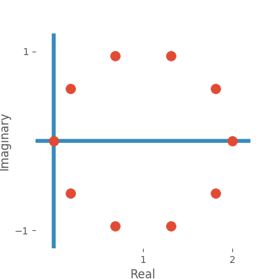
Now, this polynomial equation of order \(N\) has a fairly straightforward set of solutions for \(\lambda\): they are the roots of unity, shifted along the positive \(x\)-axis by one.

We can write the solution for \(\lambda_k\) explicitly

which, when plotted (for \(N=10\)), gives the following:

Hey, look at that! The real part of each eigenvalue is greater than zero!¹ That is to say, not only is the system unstable, it is wildly unstable. Remember, the system is unstable if if just one of the eigenvalues has a positive real part.

Simulating bus bunching

That was a long way to go, but by determining that the eigenvalues of the system of equations \eqref{perturb} all have nonnegative real parts, we determined that any perturbation to our equilibrium solution is unstable. Therefore, if any of the buses on our bus route get slightly off schedule, they will continue to get further and further off schedule.

Let's close out the article with some interactive simulations of bus bunching. The simulations start with a number of buses in the equilibrium configuration, but as you will see, they soon drift away from that equilibrium, and once they start to drift, bunching is inevitable.

There are two versions of the simulation: one in the \(v_e\) reference frame, where we see the velocities of the buses relative to their equilibrium velocity, and one in the street frame, where we see the velocities of the buses relative to the road.

In the \(v_e\) reference frame:

In the street reference frame:

Conclusion

The model we analyzed here was probably about as simple as it could be while still exhibiting bunching behavior. We used a simplified geometry, and it really only had two parameters (\(v_0\), the speed in the absence of passengers, and \(\gamma\), the amount by which passenger boarding slows it down). Nevertheless, it demonstrates a plausible mechanism for an all-too familiar occurrence for transit riders.

The good news is that actual bus system behavior can be more complex than this simple model: it has drivers, schedulers, and real-time information. It is possible to design things to mitigate the essential bunchiness of a route. Things like streamlined passenger boarding, signal priority, and layovers all likely have a role in mitigating bunching.

So what's the moral here? I'd like to say that you shouldn't feel frustrated the next time a pack of buses roll up to your stop, but that's probably not realistic. Instead, maybe just look at them with grim recognition.